Regression Analysis of of hours worked by women in 1975

The dataset Hours is a subset of the 1976 Panel Study of Income Dynamics (PSID) that contains 19 variables. In this project I will build a model that explains the number of hours worked by women in 1975. The dependent variable here is “hours”. Models with dependent variables that contain many 0’s are not usually estimated by OLS, but we ignore it for this project.

All the code and data can be found here: Github

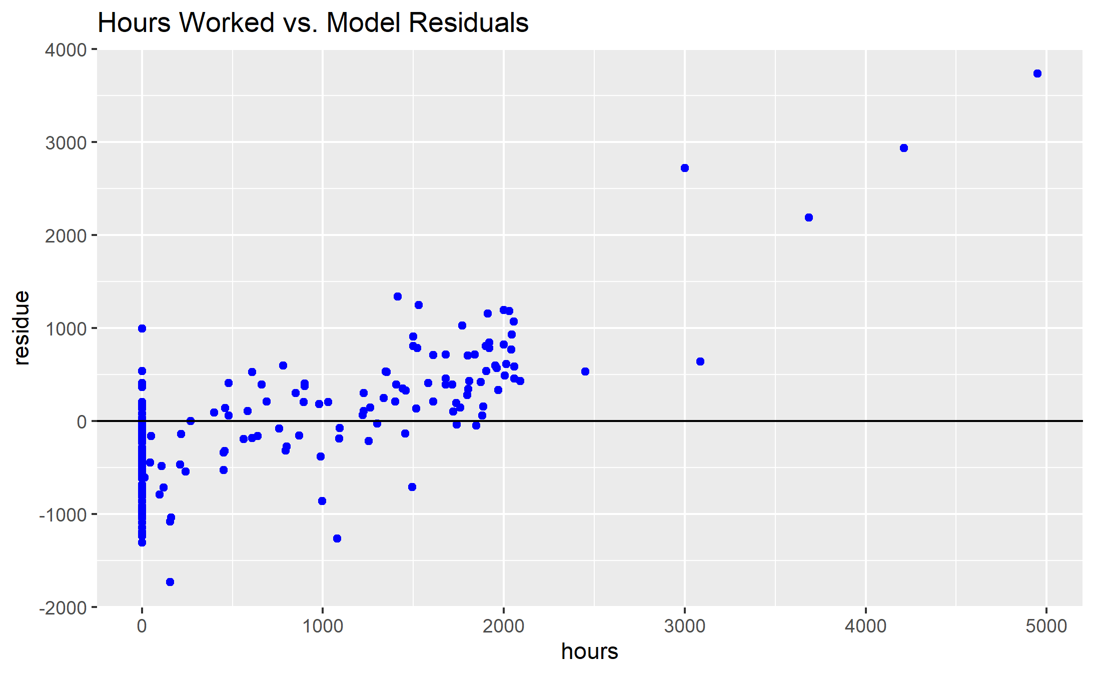
Weighted Least Squares (WLS) can be used when the data is heteroscedastic (but uncorrelated). Here since the errors are spread equally around the regression line we can see that it is not heterscedastic and so OLS is fine here.

Model Building

Variables included in the model and why

Before I can build our model, I need to decide which variables to include. I want the model to explain the number of hours worked by women in 1975. So I would need to consider whether the women had kids. If she had young kids, clearly she would probably have had to stay home to take care of them so would not have been able to work or work less hours. So I need to include the first variable “youngkids”. Note that the second variable also talks about the number of kids she had but the only difference is that the “youngkids” is the number of children less than 6 years old in household whereas “oldkids” is the number of children between ages 6 and 18 in household. Having a kid younger than 6 years old would definitely require the mother to stay home more but so would a 8 year old using same logic. So including these two variable seem redundnt and instead I will create a dummy variable of our own that is 1 if she had kids younger than 18 and 0 otherwise. We will call this variable “haveKids”. I added both youngkids and “havekids” since “youngkids” is giving the number of under 6 year old kids whereas “havekids” is a dummby variable for is she had kids at all or not.

We will have 2 groups - Woman with kids Vs Woman with no kids

Age of the woman clearly has an effect on the hours she can work. Certain jobs could be labour intensive, so the younger the woman is, the more huours she can put in. Moreover, An older woman might be more likely to be working full-time whereas an young woman might be doing a part-time job. So I decided to include this in my model.

If the woman is highly educated, she will clearly more likely to have a stable job, whereas, if the woman was not that well-educated, she would probably not be working at a stable job with “good” hours. So I thought of including “eductaion” in my model since education seem to have an effect on the number of hours worked. However, there is another varable called “college” which says “yes” is she attended college and “no” otherwise. Both are good variables to indicate the likely of the woman getting a job. However, we are more concerned with how many hours she worked, not trying to find if she had a job. So I excluded them both.

“experience” is the actual years of wife’s previous labor market experience. Higher expeirence means she is more likely to have a job and probably a good one with stable hours. So I decided to include this in my model.

“unemp” is the unemployment rate in county of residence, in percentage points. So this would gives us an idea of the demand and supply of the labor force. “city” tells us if the individual lives in a large city or not. Both “city” and “unemp” tell us if the wife had a job or not -“emp” more so than “city”. We are more concerned with how many hours she works once she already had the job, so theses two variables were not included.

“fincome” is the family income, in 1975 dollars. This would include the amount earned by both the husband and the wife. A higher “fincome” could be due to higher wage earned by the husband or the wife. “fincome” is clealry correlated with “wage”,”hhours”,”hwage”. Including all these will create some multicollinearity. “fincome” is correlated with number of hours worked by the woman too, since, the more she worked the more the “fincome” would be. We need each variable to be independant so we cannot include this in our model since we have “hwage”,”hhours” and “wage”. We must include “hhours” since clearly if the husband is woking more hours, the wife needs to stay home to take care of the family, specially in 1975. If the family didnot have kids, the wife could still decide to work less or no hours if the husband is already working a lot hours or has high wage and thus earning enough for the family. Moreover, a small “hhour” and “hwage” value might imply that wife needs to work more hours to support the family. So including all the terms as well as fincome seems redundant. I decided to skip fincome and include “hwage” and “hhours”.

fincome seemed to have some measurement error.

“tax” is the Marginal tax rate facing the wife. Since it is the marginal rate, it doesnot really help us with the hours she worked. So I excluded that as well.

To summarise, I included “havekids”,”age”,”youngkids”,”experience”,”hwage” and “hhours” in my model.

Considering 3 models (trying out log-lin, lin-lin, square variables, interactions etc.)

Once I have selected my variables, I will try 3 different models.

If the woman had kids younger than 18 at home, she might decide to stay home to take care of them or work less hours.This is also dependant on whether the husband is working long hours. If “hhours” is high the wife with kids might have to work less or no hours since you need atleast one parent to be there for the kids. So I want to introduce the interaction between “havekids” and “hhours” since I believe there is a relationship between them.

I want to try $expereince^2$. Clearly if the woman had exprience equal to sample average she will probably be working a stable job with good hours.

if the “hwage” is high the wife might decide to stay home since the husband is already providing enough money to support the family. This further increased if the husband is working more hours. So I want to see the effect of adding an interaction for hhour and hwage.

I added the interaction $havekids \times hhours$ since having kids and the husband working long hours will have an added effect on the wife’s ability to work.

I tried $log(hours)$ to make sure the residuals are not too skewed. I have both $havekids \times hhours^2$ and hhours, since there is likely to things how the husband’s working hours effects the wife’s: 1. Having kids and housband working long hours will result in wife deciding to work less hours to stay home and take care of the kids, 2. Husband woring long hours and so earning enough to support the family.

The first model is:

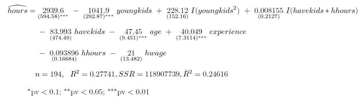
The second model is:

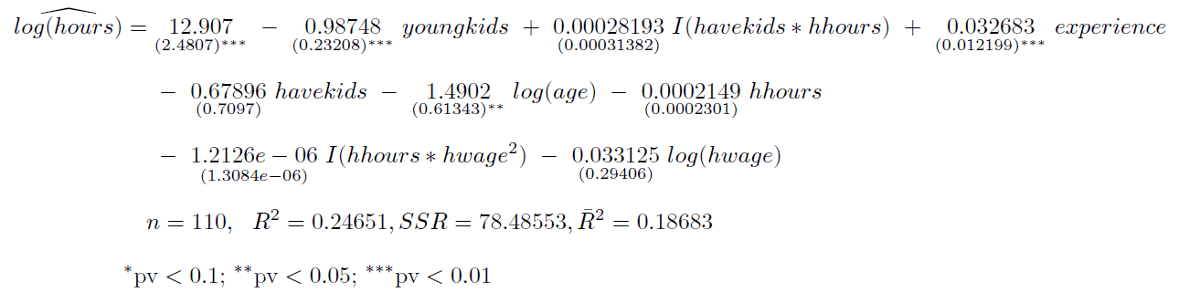
The third model is:

We first estimate the models and test the homoscedasticity using the short White test:

Checking model_1:

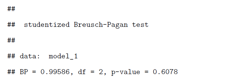
Since p-value is greater than 0.05, we do not reject the homoscedasticity assumption at 5%, so we do not need to use robust tests.

Checking model_2:

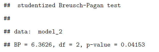
Since p-value is less than 0.05, we reject the homoscedasticity assumption at 5%, so we need to use robust tests.

Checking model_3:

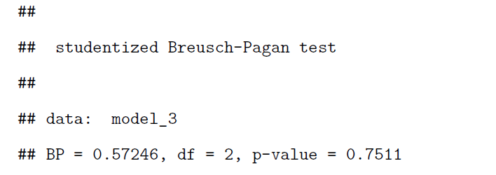
Since p-value is greater than 0.05, we do not reject the homoscedasticity assumption at 5%, so we do not need to use robust tests.

Model_1 and Model_3 are nested models.So we can just use indirect-t test to see if the extra “youngkids^2” term is significant or not in model 1.

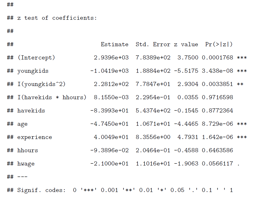
Since p-value is less than 0.05 we reject the Null hypothesis that the coefficient of “youngkids^2” is 0. So we conclude that “youngkids^2” is significant. So we choose Model 1 instead.

Now we need to choose between the two non-nested models: Model_1 and Model_2. We need to use robust J-test for that since model 2 is heteroscedastic:

J test

Model 1: hours ~ youngkids + I(youngkids^2) + I(havekids * hhours) + havekids +
    age + experience + hhours + hwage
Model 2: log(hours) ~ youngkids + I(havekids * hhours) + experience +
    havekids + log(age) + hhours + I(hhours * hwage^2) + log(hwage)
                Estimate Std. Error z value Pr(>|z|)
M1 + fitted(M2)   0.6909    0.91397  0.7559   0.4497
M2 + fitted(M1)   1.7307    1.77742  0.9737   0.3302

Both have p-value greater than 0.05 so we can see that both models cannot be rejected. I decided to go with mdoel 1 because choosing model 2 will result in us losing a lot of data (we lose all the data corresponding to hours less than or equal to 0).

Now I will test the null hypothesis that the model is correctly specified at 5% using the RESET test. Since it is homoscedastic, we can just use the non-robust test.

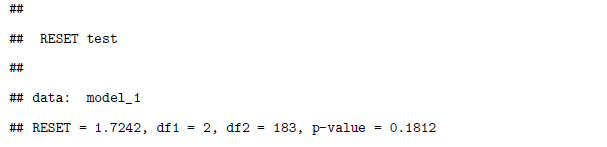
The p-value is greater than 5% we cannot reject the hypothesis that the model is correctly specified.

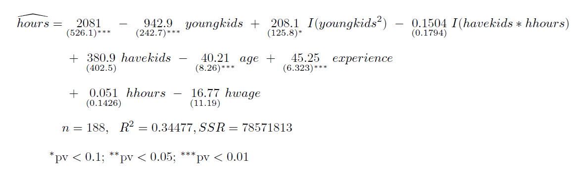
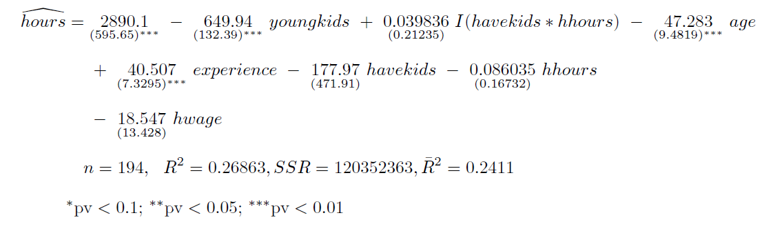
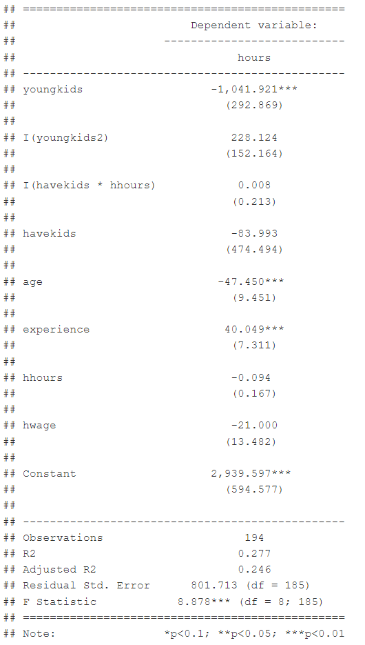
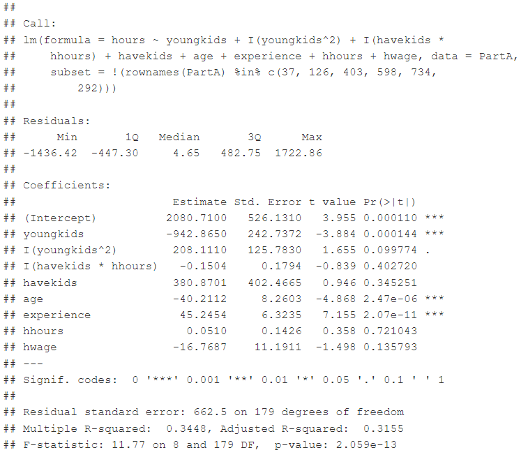
The summary for Model 1 is as follows:

Removing Outliers

The Cook’s distance for detecting outliers is plotted by the plot method for lm objects.

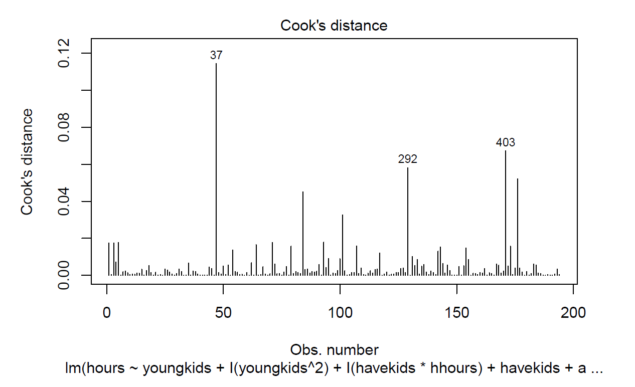
These are the names of the rows (37,403,126).So we can remove observations 126, 403 and 37.

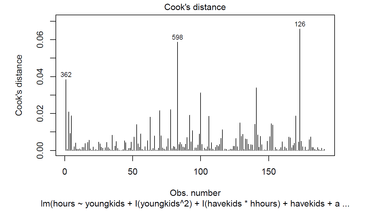
There seem to still be some outliers. Removing those too:

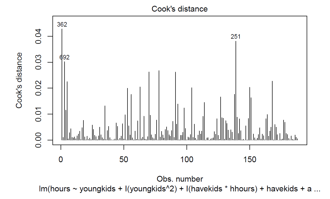
Now, the Cook’s distance are closer to being equal. We can compare the results to see what is the impact of dropping these three observations:

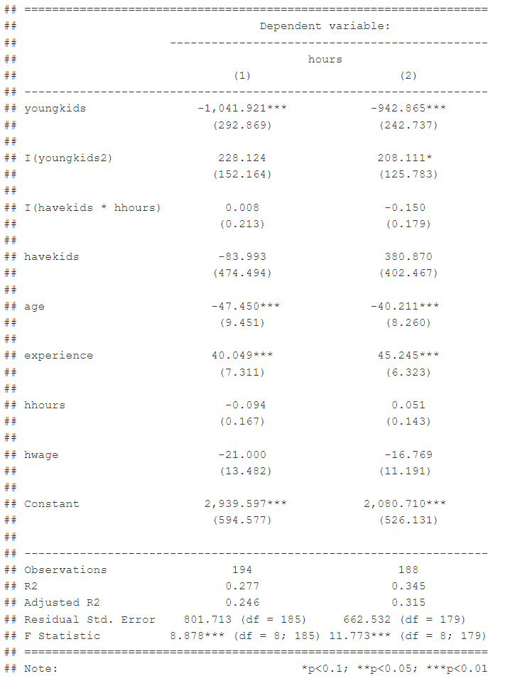
Interpretation and Analysis

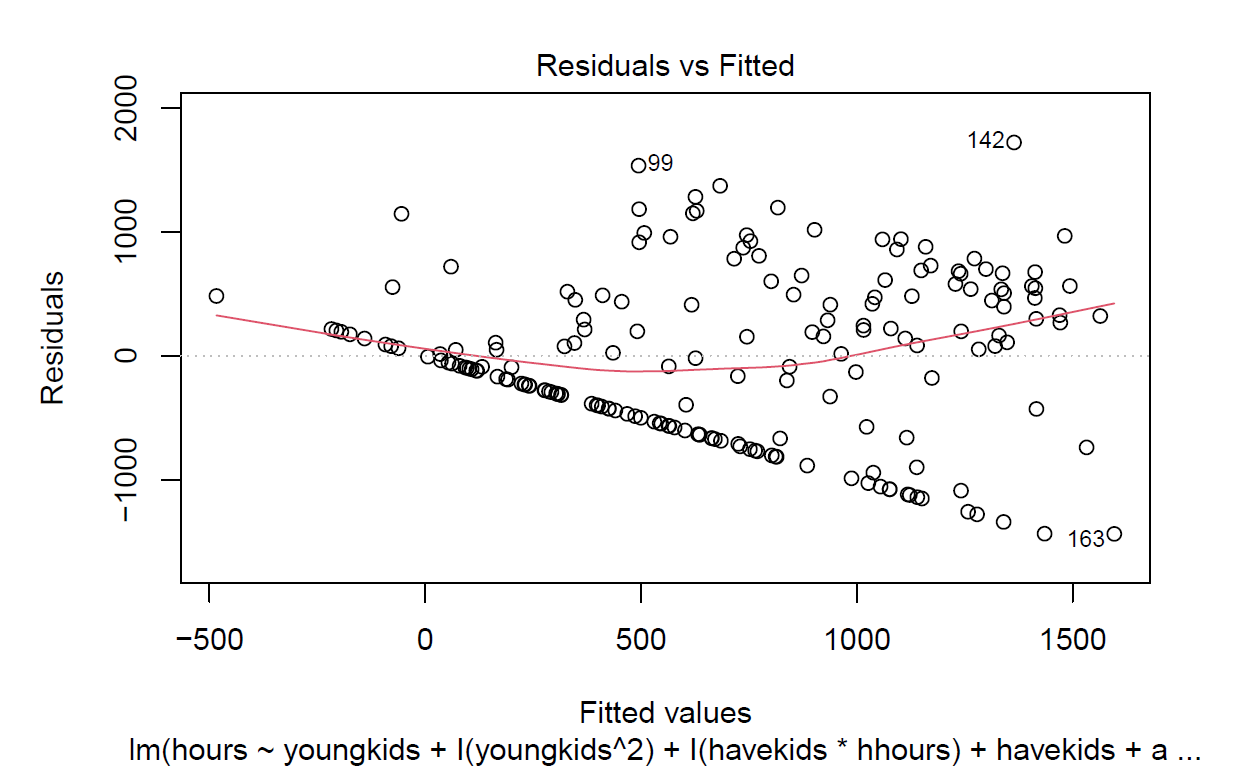
Since model 1 is homoscedastic we can just use summary() to check the coefficients:

Interpreting the coefficients

Intercept: Here the intercept has no meaning since age would have to be 0 which has no meaning.

youngkids and $youngkids^2$ need to be explained using partial effect which is done in the next section.

age: women who are 1 more year older will have a difference in hours worked of 40.2112 less when holding all the other variables constant.

experience: women who have 1 more year of experience will have a difference in hours worked of 45.2454 more when holding all the other variables constant.

hwage: women whose husbands earn 1 more dollar in wage will have a difference in hours worked of 16.7687 less when holding all the other variables constant.

For hhours and $havekids \times hhours$

If the woman had no kids the difference in hours worked will be 0.0510 more when holding all the other variables constant. But, if the woman had kids the difference in hours worked will be 0.0994 less when holding all the other variables constant.

Significance of the coefficients

Firstly, p-value of I(youngkids^2) is greater than 0.05, so we cannot reject Null Hypothesis. So we can say that the relationship is linear.

youngkids,age and experience are the only statisticall significant features in this model since they have p-value less than 0.05 (so we can reject Null Hypothesis.)

Confidence Interval of the coefficients

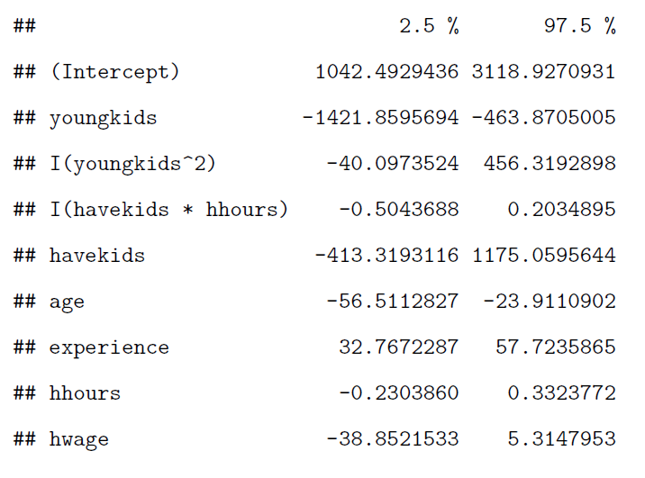
These intervals are where we will find its corresponding variables 95% of the time.

Average partial effects:

average partial effect of youngkids on hours is $\beta_1+2\beta_2\overline{youngkids}$

The average hours worked by the woman with a kid yonger than 6 and the same level of education, hhours,age and hwage is 857.0461 hours less, when their initial number of young kids is equal to the sample average.

95% of the time the true APE is between -1247.563 and -466.529

Hypothesis Testing

Does having children less than 6 have the same effect as having children between ages 6 and 18?

The model is:

if the woman has children less than 6, then we can use this model for inference however, if the woman doe not have children less than 6 but instead only has children between ages 6 and 18, then youngkids = 0 but havekids is still 1. So our new model would be:

I want to see if $\beta_1=\beta_2=0$

Using F-test (non-robust since it is homoscedastic):

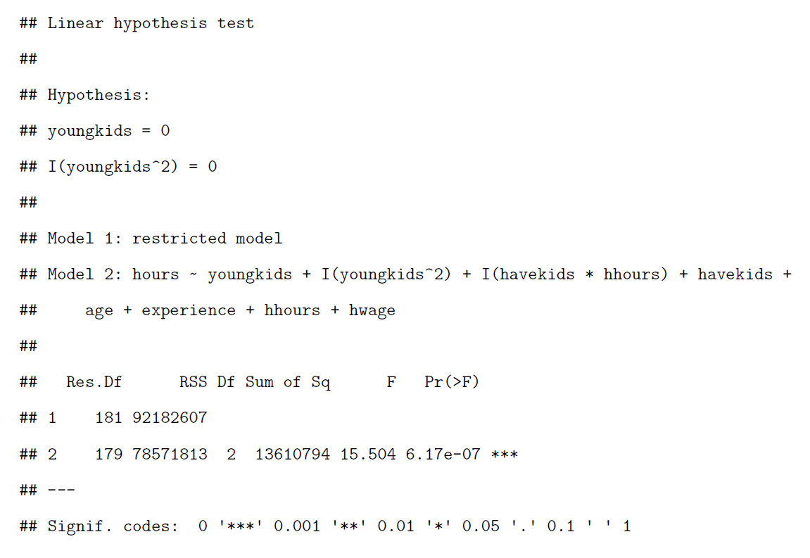
Since p-value is less than 0.05 we can reject the Null hypothesis and conclude that having children less than 6 does not have the same effect as having children between ages 6 and 18.

Effect of youngkids and hhours

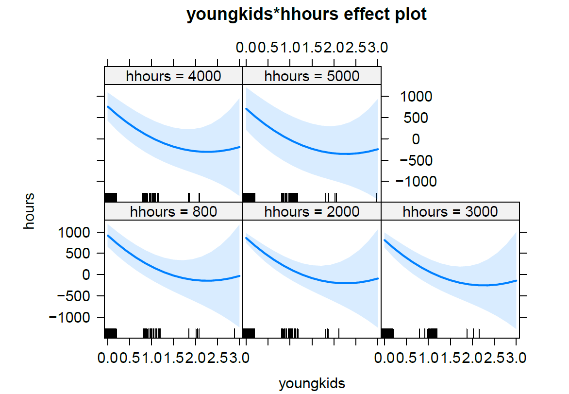
hhours and youngkids seem to have an inverse non linear relationship

WOMEN WITHOUT KIDS VS WOMEN WITH KIDS

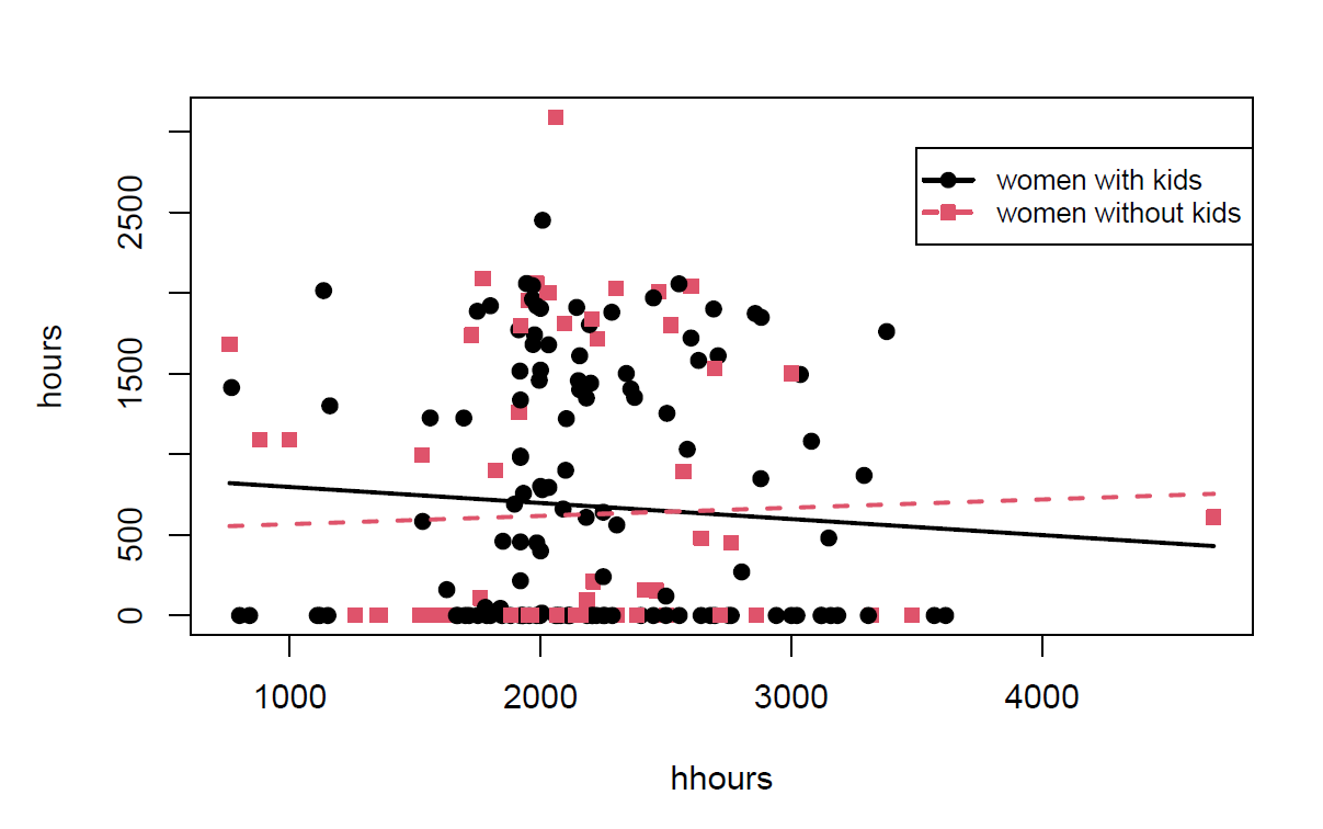
Looking at the above graph, we can see that initially when the husband is working less hours (approximately less than 2500 hours), the wife with kids is working more hours but then we see after around 2500 hhours, the women with kids have their wroking hours reduce, implying that as the husband works more hours, the wife decides to work less hours if she had kids. On the other hand, we see an oopsite trend for women without kids,where as hhours increase so does the wife’s working hours.

Hence the final model is: